Topological structure (network): Difference between revisions
| [checked revision] | [checked revision] |
mNo edit summary |
No edit summary |
||
| Line 38: | Line 38: | ||
The next step adds the routing information to produce the optimised connexity representation. | The next step adds the routing information to produce the optimised connexity representation. | ||
Considering the initial diagram and using the knowledge about the switch depicted as node B it possible to enrich the current diagram with explicit navigability information at the relations: | Considering the initial diagram and using the knowledge about the switch depicted as node B it possible to enrich the current diagram with explicit navigability information at the relations:<br /> | ||
[[File:NavigabilityInformationRel.png]] | [[File:NavigabilityInformationRel.png]] | ||
| Line 49: | Line 49: | ||
These relations are expressed more compactly using a matrix: | These relations are expressed more compactly using a matrix: | ||
[[File:RelationsMatrix.png]] | [[File:RelationsMatrix.png]] | ||
The physical view is not very well suited for a specific class of use cases like routing, timetabling or simulation. | |||
With physical relations matrix alone, it is impossible to tell that, through B, it is not allowed to go from 3 to 2, as there is no direct relation between 3 and 2. | |||
In fact, all the connections to and from a node are always navigable, as it means that a train can “enter” the node from there. | |||
So the “Physical” level is complemented with a “Functional”, or routing level describing how the elements act together as a routable network. | |||
To know the relations between the objects through one node, the interactions between the elements are described related to that node. So the relations between the following elements are shown: | |||
[[File:Navigability.png]] | |||
Many existing datasets covering the physical view contain information objects which are not essential for routing algorithms. These objects increase the address space as well as the runtime of algorithms. The table below shows the most common nodetypes of railway networks at the micro description level. | |||
{| class="wikitable" | |||
|- | |||
! Micro level nodetypes !! Number of neighbours !! Type of neighbours | |||
|- | |||
| bufferstop || 1 || trackEdge | |||
|- | |||
| borderpoint || 1 || trackEdge | |||
|- | |||
| switch || 3 || trackEdge, adjacent switch or crossing | |||
|- | |||
| Double Diamond Crossing || 4 || trackEdge, adjacent switch or crossing | |||
|- | |||
| Single Diamond Crossing || 4 || trackEdge, adjacent switch or crossing | |||
|- | |||
| crossing || 4 || trackEdge, adjacent switch or crossing | |||
|- | |||
| turntable || depending on construction || trackEdge | |||
|- | |||
| Transfer table || depending on construction || trackEdge | |||
|} | |||
All those elements above can be removed from the dataset provided that the linear elements (pieces of track between two nodes aka trackEdge) carry the necessary attributes for navigation.<br /> | |||
In the RailTopoModel the navigability information can be stored in an optimal way at the PositionedRelation between the edges of the respective level.<br /> | |||
If there exists a connected dataset with the NetElements and Relations below the current description level, navigability can be deduced from this information. The micro level data without navigability information together with nano level data containing the topological structure of each switch, crossing, turntable or transfer table allow to transfer navigability information to the micro level. After removal of the superfluous nodes the resulting subset of micro level data consists only of trackEdges with the relevant navigability information which in turn is relevant to routing algorithms.<br /> | |||
In case the detailed nano level information does not yet exist, it is also quite easy to add navigability information manually directly to the trackEdges.<br /> | |||
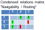
The RailTopoModel provides the necessary structures to produce a condensed relation matrix out of the detailed physical relations matrix. If there exists a detailed nano level description of each switch connected to the micro level – as is the case in some pilot projects of early adopters of the RailTopoModel – then full automation is achievable.<br /> | |||
The same principle holds true between the macro and the micro level. This again is a direct consequence of the elegant recursive nature of the RailTopoModel. | |||
[[File:CondensedMatrix.png]] | |||
Revision as of 11:02, 24 March 2016
|
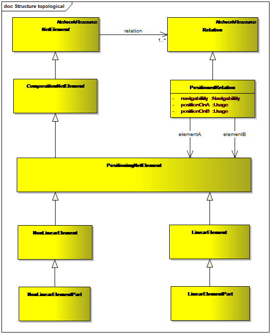
The topological structure of the network describes the relations of the building blocks of the network in the context of a given description level.
The class “NetElement” depicts all building blocks of the topology. In a classical physical description it consists of what is commonly called “nodes” and “edges”. In the optimised description for fast operational computations the physical nodes are removed and only the edges remain. The properties of the physical nodes are the basis for the relations. A detailed description of the conversion from the classical description into the optimised connexity based description can be found below.
Therefore the class “PositionedRelation” which is inheriting the associations to “NetElement” contains attributes which describe navigabilty as well as hints for the position at the associated “PositioningNetElements”.
The classes “LinearElement” and “LinearElementPart” serve for anchoring localisations of “NetEntity” instances via “AssociatedNetElement”.
The classes “NonLinearElement” and “NonLinearElementPart” serve for anchoring localisations of “NetEntity” instances via “SpotLocation”.
Based on this structure of the topological network description the following diagrams show the interaction of the “NetElement” instances. That interaction provides the glue to use those components as a network.
The sample network consists of four nodes and three edges and is shown in a classical physical representation.
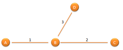
In RailTopoModel those four nodes and three edges are represented as seven “NetElement” instances shown in the “Network element view”.
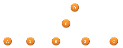
This pure “NetElement” view misses the topological relations of the original classical representation. Therefore “Relation” instances are added which represent the topological connections. Each “Relation” instance connects two “NetElement” instances.
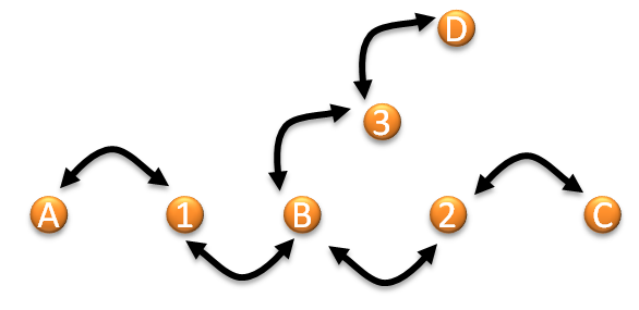
An association between linear “NetElement” instances and a “Relation” instance requires the information at which end of the linear object the relation is valid. This information can be found in the specialised class “PositionedRelation”. The two attributes “positionOnA” and “positionOnB” contain location information using intrinsic coordinates. “0” means that the relation is located at the beginning of the “NetElement” instance, “1” means that the relation is located at the end of the “NetElement” instance.
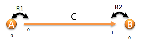
The relation “R1” carries the following information:
- ElementA : element named A
- PositionOnA : 0 (non linear element)
- Element B : element named C
- PositionOnB : 0 (start of the element)
The relation “R2” carries the following information :
- ElementA : element named C
- PositionOnA : 1 (end of the element)
- Element B : element named B
- PositionOnB : 0 (non linear element)
So far the graph expresses the connectedness of the elements.
The next step adds the routing information to produce the optimised connexity representation.
Considering the initial diagram and using the knowledge about the switch depicted as node B it possible to enrich the current diagram with explicit navigability information at the relations:
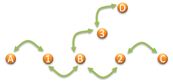
Meaning :
- It is possible to go from A to 1 (and vice versa)
- It is possible to go from 1 to B
- It is possible to go from B to 3
- It is possible to go from B to 2
- …
These relations are expressed more compactly using a matrix:

The physical view is not very well suited for a specific class of use cases like routing, timetabling or simulation.
With physical relations matrix alone, it is impossible to tell that, through B, it is not allowed to go from 3 to 2, as there is no direct relation between 3 and 2.
In fact, all the connections to and from a node are always navigable, as it means that a train can “enter” the node from there.
So the “Physical” level is complemented with a “Functional”, or routing level describing how the elements act together as a routable network.
To know the relations between the objects through one node, the interactions between the elements are described related to that node. So the relations between the following elements are shown:
 Many existing datasets covering the physical view contain information objects which are not essential for routing algorithms. These objects increase the address space as well as the runtime of algorithms. The table below shows the most common nodetypes of railway networks at the micro description level.
| Micro level nodetypes | Number of neighbours | Type of neighbours |
|---|---|---|
| bufferstop | 1 | trackEdge |
| borderpoint | 1 | trackEdge |
| switch | 3 | trackEdge, adjacent switch or crossing |
| Double Diamond Crossing | 4 | trackEdge, adjacent switch or crossing |
| Single Diamond Crossing | 4 | trackEdge, adjacent switch or crossing |
| crossing | 4 | trackEdge, adjacent switch or crossing |
| turntable | depending on construction | trackEdge |
| Transfer table | depending on construction | trackEdge |
All those elements above can be removed from the dataset provided that the linear elements (pieces of track between two nodes aka trackEdge) carry the necessary attributes for navigation.
In the RailTopoModel the navigability information can be stored in an optimal way at the PositionedRelation between the edges of the respective level.
If there exists a connected dataset with the NetElements and Relations below the current description level, navigability can be deduced from this information. The micro level data without navigability information together with nano level data containing the topological structure of each switch, crossing, turntable or transfer table allow to transfer navigability information to the micro level. After removal of the superfluous nodes the resulting subset of micro level data consists only of trackEdges with the relevant navigability information which in turn is relevant to routing algorithms.
In case the detailed nano level information does not yet exist, it is also quite easy to add navigability information manually directly to the trackEdges.
The RailTopoModel provides the necessary structures to produce a condensed relation matrix out of the detailed physical relations matrix. If there exists a detailed nano level description of each switch connected to the micro level – as is the case in some pilot projects of early adopters of the RailTopoModel – then full automation is achievable.
The same principle holds true between the macro and the micro level. This again is a direct consequence of the elegant recursive nature of the RailTopoModel.
